Understanding Bonding Curves: From Math to Implementation

Table of Contents

Bonding curves represent one of the most fascinating intersections of mathematics and tokenomics in the web3 space. In this comprehensive guide, we’ll explore how bonding curves work, implement one in Solidity, and test it thoroughly using Foundry.

1. Mathematical Foundations

The Basic Formula

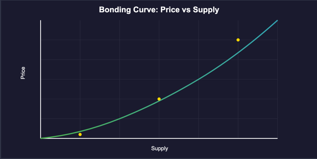
Imagine you’re designing a new token distribution mechanism. You want the price to increase as more people buy, but in a predictable way. This is where exponential bonding curves come in. A bonding curve uses the formula:

$$P = Ae^{Bx}$$

Where:

P is the token price
A is the initial price factor
B is the exponential growth factor
x is the current supply
e is Euler’s number (≈ 2.71828)

Let’s make this concrete with an example. If we set A to 0.000001 (or 1e6 in code), our token starts at a mere fraction of a dollar - perfect for early adopters. The B parameter requires more careful consideration; too high and prices become prohibitive quickly, too low and the price barely moves.

Understanding Each Component

Initial Price Factor (A)

The initial price factor A is fundamental to your token’s accessibility and adoption strategy. It determines the starting point of your bonding curve:

$$P = Ae^{Bx} \text{ at } x = 0, \text{ therefore } P = A$$

Let’s break down what different A values mean in practice:

If A = 0.000001 (1e6):
- Initial token price = 0.000001 USDC
- First 100 tokens would cost approximately 0.0001 USDC
- Great for community projects wanting wide participation
If A = 0.001 (1e3):
- Initial token price = 0.001 USDC
- First 100 tokens would cost approximately 0.1 USDC
- Balanced approach for most projects
If A = 0.1 (1e1):
- Initial token price = 0.1 USDC
- First 100 tokens would cost approximately 10 USDC
- Suitable for premium or limited supply tokens

Choosing A requires balancing several factors:

Target Audience: Lower A values make early participation more accessible
Spam Prevention: Very low A values might invite spam transactions
Initial Capital: Higher A values require more capital to participate
Market Positioning: A signals your token’s initial perceived value

Growth Factor (B)

The growth factor B is your curve’s “sensitivity” parameter. It determines how aggressively prices change with supply. For prices P₁ and P₂ at supplies x₁ and x₂:

$$\frac{P_2}{P_1} = e^{B(x_2-x_1)}$$

Let’s analyze different B values with concrete examples:

Gentle Slope (B = 0.0000001 or 1e7)

Initial price: 0.000001 USDC
After 1,000 tokens: 0.0000011 USDC (+10%)
After 10,000 tokens: 0.0000020 USDC (+100%)

Best for: Long-term accumulation, stable growth projects

Moderate Growth (B = 0.000001 or 1e6)

Initial price: 0.000001 USDC
After 1,000 tokens: 0.0000027 USDC (+170%)
After 10,000 tokens: 0.0000148 USDC (+1,380%)

Best for: Balanced tokenomics, medium-term projects

Aggressive Growth (B = 0.00001 or 1e5)

Initial price: 0.000001 USDC
After 1,000 tokens: 0.0000148 USDC (+1,380%)
After 10,000 tokens: 0.0022026 USDC (+220,160%)

Best for: Highly speculative or scarce-by-design tokens

Considerations when choosing B:

Market Depth: Higher B values create deeper markets faster
Price Sensitivity: Higher B means more volatile prices
Whale Impact: Higher B makes large purchases more expensive
Long-term Viability: Lower B supports sustainable growth

Price Discovery Mechanism

The bonding curve creates an automated market maker (AMM) with unique properties. Let’s examine the buy and sell mechanics:

Buying Tokens

When users buy tokens, several mathematical processes occur:

Supply Increase: The new supply affects price according to our base formula:
$$P = Ae^{Bx}$$
Price Calculation: For any purchase, we calculate the average price by integrating over the supply range:
$$\text{Average Price} = \frac{1}{x_1-x_0}\int_{x_0}^{x_1} Ae^{Bx} \, dx$$
Cost Determination: The total cost for purchasing tokens is the integral of the price function:
$$\text{Total Cost} = \int_{x_0}^{x_1} Ae^{Bx} \, dx$$
Which evaluates to:
$$\text{Cost} = \frac{A}{B}(e^{Bx_1} - e^{Bx_0})$$

Selling Tokens

The sell mechanism mirrors buying but with important distinctions:

Supply Decrease: The supply reduction affects the price according to:
$$\text{New Supply} = \text{Current Supply} - \text{Sell Amount}$$
Price Impact:

Selling follows the same curve in reverse
Each token sold receives slightly less than the previous
The average sell price is lower than the spot price

Slippage Calculation:
$$\text{Slippage} = \frac{P_{\text{spot}} - P_{\text{avg}}}{P_{\text{spot}}} \times 100\%$$

Example Sell Scenario:

Current Supply: 10,000 tokens
Spot Price: 0.01 USDC
Sell Amount: 1,000 tokens
Average Sale Price: ~0.0095 USDC
Slippage: ~5%

This mechanism creates several important properties:

Instant Liquidity: Always available at a calculable price
Price Discovery: Market forces directly affect token price
Slippage Protection: Large trades have predictable impact
Arbitrage Opportunities: Helps maintain price equilibrium with external markets

Integration and Areas

To calculate actual token amounts and costs, we need calculus. When someone buys tokens:

$$\text{Total Cost} = \int_{x_0}^{x_1} P \, dx$$

This translates to:

$$\text{Cost} = \frac{A}{B}(e^{Bx_1} - e^{Bx_0})$$

2. Implementation Setup

First, let’s set up our development environment and break down the implementation step by step.

Setting Up Foundry

Create a new project and install dependencies:

forge init bonding-curve
cd bonding-curve
forge install vectorized/solady

Project Structure

bonding-curve/
├── src/
│   └── BondingCurve.sol
├── test/
│   └── BondingCurve.t.sol
└── lib/
    └── solady/

Core Contract Implementation

Let’s break down our BondingCurve.sol contract piece by piece:

1. Contract Setup and Dependencies

// SPDX-License-Identifier: MIT
pragma solidity ^0.8.13;

import "solady/utils/FixedPointMathLib.sol";

contract BondingCurve {
    using FixedPointMathLib for uint256;
    using FixedPointMathLib for int256;

We’re using Solady’s FixedPointMathLib for efficient fixed-point arithmetic operations.

2. State Variables and Constants

    /// @notice Initial price factor (A in the formula)
    uint256 public immutable A;

    /// @notice Exponential growth factor (B in the formula)
    uint256 public immutable B;

    /// @notice Maximum allowed supply
    uint256 public constant MAX_SUPPLY = 10_000_000e18; // 10M tokens

    /// @notice Maximum transaction size
    uint256 public constant MAX_TX_SIZE = 1_000_000e18; // 1M tokens

    /// @dev Maximum exponent allowed
    int256 public constant MAX_EXP_VALUE = 50e18;

    /// @dev Minimum remaining supply
    uint256 public constant MIN_REMAINING_SUPPLY = 1000e18;

These constants define our curve’s boundaries and safety limits.

3. Custom Errors

    error SupplyExceedsMaximum(uint256 supply, uint256 maximum);
    error TransactionTooLarge(uint256 size, uint256 maximum);
    error ExponentTooLarge(int256 value, int256 maximum);
    error InsufficientRemainingSupply(uint256 remaining, uint256 minimum);

Using custom errors for gas-efficient error handling and better debugging.

4. Constructor

    constructor(uint256 _a, uint256 _b) {
        require(_a > 0, "A must be positive");
        require(_b > 0, "B must be positive");
        A = _a;
        B = _b;
    }

Initializes our curve parameters with basic validation.

5. Core Mathematical Functions

Price Calculation

    function getCurrentPrice(uint256 x) public view returns (uint256 price) {
        if (x > MAX_SUPPLY) {
            revert SupplyExceedsMaximum(x, MAX_SUPPLY);
        }

        int256 exp_b_x = int256(B.mulWad(x));
        _checkExponent(exp_b_x);
        price = A.mulWad(uint256(exp_b_x.expWad()));
    }

Implements our price formula using fixed-point math.

Buy Amount Calculation

    function getAmountOut(
        uint256 x0,
        uint256 deltaY
    ) public view returns (uint256 deltaX) {
        uint256 remainingSupply = MAX_SUPPLY - x0;
        if (remainingSupply < MIN_REMAINING_SUPPLY) {
            revert InsufficientRemainingSupply(
                remainingSupply,
                MIN_REMAINING_SUPPLY
            );
        }

        // Calculate e^(B*x0)
        int256 exp_b_x0 = int256(B.mulWad(x0));
        _checkExponent(exp_b_x0);

        // Calculate e^(B*x0) + (deltaY*B/A)
        uint256 exp_b_x1 = uint256(exp_b_x0.expWad()) + 
            deltaY.fullMulDiv(B, A);

        // Calculate (ln(exp_b_x1)/B) - x0
        deltaX = uint256(int256(exp_b_x1).lnWad()).divWad(B) - x0;

        if (deltaX > MAX_TX_SIZE) {
            revert TransactionTooLarge(deltaX, MAX_TX_SIZE);
        }
    }

Calculates tokens received for a given payment amount using integral calculus. You can get the complete code on my GitHub .

Testing Setup

Create BondingCurve.t.sol with basic test parameters:

contract BondingCurveTest is Test {
    using FixedPointMathLib for uint256;
    using FixedPointMathLib for int256;

    BondingCurve public curve;

    // Test parameters
    uint256 constant A = 1e6;    // 0.000001 USDC starting price
    uint256 constant B = 1e12;   // 0.000001 growth rate

    function setUp() public {
        curve = new BondingCurve(A, B);
    }
}

Key Implementation Notes

Fixed-Point Math: We use WAD (18 decimals) precision throughout for consistent calculations.
```
// Example: mulWad for multiplication
price = A.mulWad(uint256(exp_b_x.expWad()));
```
Safety Checks: Each function includes bounds checking:

Supply limits
Transaction size limits
Exponent overflow prevention
Minimum remaining supply

Gas Optimization:

Using custom errors instead of require statements
Immutable state variables where possible
Efficient math library from Solady

Precision Handling:

// Helper function for comparing values with precision
function assertAlmostEqual(
    uint256 a, 
    uint256 b, 
    uint256 precision
) internal {
    if (a > b) {
        uint256 diff = a - b;
        assertTrue(
            diff <= precision, 
            "Values differ by more than precision"
        );
    } else {
        uint256 diff = b - a;
        assertTrue(
            diff <= precision, 
            "Values differ by more than precision"
        );
    }
}

Running Tests

Execute the test suite:

forge test -vv

This will run all test cases with verbose output, showing the progression of values through our bonding curve implementation.

3. Testing and Validation

Key Test Scenarios

1. Price Progression

We test price increases across different supply points:

function testPriceGrowthRate() public {
    // Supply points: 1K, 10K, 100K, 1M, 5M tokens
    // Verifies exponential growth pattern
}

2. Buy/Sell Symmetry

Important for fair market dynamics:

function testBuySellSymmetry() public {
    // Should get approximately same amount when buying/selling
    // Small difference due to precision is acceptable
}

Numerical Limitations

Our testing revealed critical limitations:

Exponential Overflow

Large supplies cause exponential calculations to overflow
Required reducing MAX_SUPPLY to 10M tokens
Added explicit bounds checking

Precision Loss

Small numbers need careful handling
Used WAD (1e18) precision throughout

4. Practical Considerations

Gas Optimization vs Safety

Our implementation prioritizes safety over gas efficiency:

Added Checks

if (remainingSupply < MIN_REMAINING_SUPPLY) {
    revert InsufficientRemainingSupply(remainingSupply, MIN_REMAINING_SUPPLY);
}

Parameter Bounds

MAX_SUPPLY = 10_000_000e18
MAX_TX_SIZE = 1_000_000e18
MAX_EXP_VALUE = 50e18

Economic Implications

The bonding curve creates interesting economic dynamics:

Early Adopter Advantage

Earlier buyers get lower prices
Creates natural incentive for early participation

Price Stability

Large buys cause exponential price increases
Discourages market manipulation

Liquidity Guarantee

Contract always provides buy/sell liquidity
Price is deterministic and transparent

5. Advanced Topics

Parameter Selection

Choosing A and B parameters requires careful consideration:

Initial Price (A)

Too low: Vulnerable to spam transactions
Too high: Barriers to entry
Recommended: 1e6 (0.000001 USDC)

Growth Rate (B)

Too low: Insufficient price movement
Too high: Price becomes prohibitive quickly
Recommended: 1e10 to 1e12

Safety Mechanisms

Our implementation includes several safety features:

Supply Caps

Prevents numerical overflow
Manages economic expectations

Transaction Size Limits

Prevents market manipulation
Ensures price stability

Remaining Supply Check

Ensures orderly market end
Prevents edge case exploitation

Conclusion

Bonding curves represent a powerful primitive for token distribution and price discovery. Our implementation demonstrates how to balance mathematical elegance with practical constraints and safety considerations.

Key takeaways:

Mathematical precision requires careful bounds
Safety checks are crucial but come with tradeoffs
Parameter selection significantly impacts behavior
Testing must cover both normal and edge cases

The future of bonding curves likely involves:

More sophisticated growth patterns
Integration with other DeFi primitives
Enhanced safety mechanisms
Optimized implementations

References

Original implementation: pump.fun
Solady library: Fixed point math
Foundry documentation: forge-std